
DRIVEN HARMONIC OSCILLATOR
References: Any Junior-level mechanics book: resonance, damped and driven harmonic motion, normal modes. Check here for motion sensor setup. Check here for curve fitting and error analysis basics.
Equipment: (not listed in its entirety)
The purpose of this experiment is to understand the dynamics of the one-dimensional driven harmonic oscillator with 1 or 2 masses. We will first consider a simple oscillator with 1 mass, no damping, and no external drive. We will then add damping and an external drive. In the end, we will explore what happens with additional masses.
The web write-up should include any work you did in Excel, MathCad, etc. In addition, you should do some background research on examples of resonance modes and why harmonic oscillators are important. Remember to read the description of what should be included in your report, and to add links to any useful web resources. As well as web research, your preliminary work could include answers to the exercises and figuring out how to fit the data in the various parts. Asample data set for the damped data is included on the class web page. If you would like pointers on data fitting, please ask me, check out the help in MathCad, Origin, or Axum, or or check out the computer hints (on class web page) for fitting in Excel.
Part 1. Simple Harmonic Oscillator
The figure below shows a glider of mass m and length lo connected by springs to two fixed points x1 and L. The springs have spring constants k1 and k2 and equilibrium lengths l1 and l2.

The forces F1 and F2 acting on m are:
(1.1) F1 = k1((x-x1)-l1) to the left.
(1.2) F2 = k2((L-(x+l0)-l2) to the right.
If we measure x relative to the equilibrium position, then the value of x at equilibrium is 0. Applying Newton's Second Law to the equilibrium problem, we can find relationships between the constants in the force equations. This simplifies the problem considerably, giving
(1.3) Fnet = -(k1+k2)x.
Now if we apply Newton's Second Law to the moving cart, displaced from equilibrium and left free to roam, we find
(1.4) mx'' = -(k1+k2)x,
where x'' indicates second derivative of displacement (i.e. acceleration).
This is a straight forward differential equation. Guessing a solution, we find that
(1.5) x = Asin(
w0t + f)works as long as
(1.6)
w0 = ((k1 + k2))/m)1/2.Experiment 1A. Measure m and the spring constants k1 and k2.
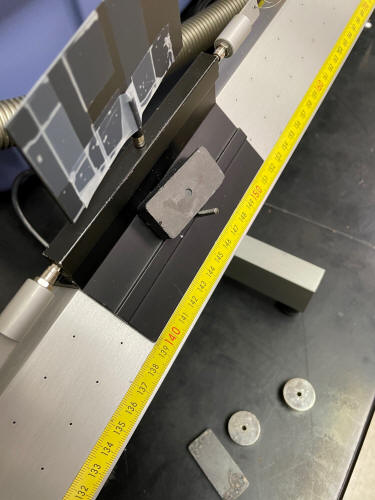
In part 2, you will need magnets for damping. So if you were to add magnets, you woudl change the mass and change the frequency of osciallation. Since we want to keep the mass consistent between trials, to keep that from happening, you need to add mass to the cart right now equivalent to the mass of the two magnets. The rectangular ceramic magnets we use for this are 50 g each, which is the same mass as the masses made to go on the black airtrack carts. Be sure to attach those two masses to the cart now, and later, when you use magnets, replace each mass with a magnet as needed.
Image of magnets and equivalent mass:
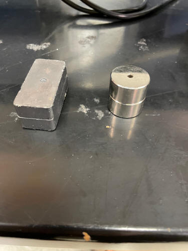
Image of mass on the cart when you do not need a magnet:
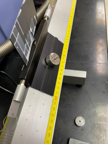
Image of mass being replaced by a magent:
The easiest way to measure the spring constants is to hang weight on each spring and measure how far it extends from some fixed point. Note that the spring constant is dF/dx, and not F/x, because of the arbitrary y-intercept of F vs. x. Therefore you want to make a precise determination of of each k by plotting F vs x. and take the SLOPE. Be sure to do appropriate error analysis.
Experiment lB. Determine the natural frequency w0 of the undamped glider and the two springs by measuring the elapsed time for 20 or more oscillations. Measure several times, compute the average and standard error. Check whether the measured w0 agrees with the expected value, w0 = ((k1 + k2)/m)1/2.
Part 2. Harmonic oscillator with damping.
If the magnets are placed on the lower part of the skirts of the glider (replacing the 50 g mass as in the third picture above), the magnetic field will extend through glider into the air track. If the glider is moving and the track is stationary, eddy currents in the track generate a velocity-dependent force = cv, which opposes the motion. The force on the glider is then
(2.1) F = - (k1 + k2)x - cx'
The differential equation describing the motion is then
(2.2) mx'' + cx' + kx = 0
The solution to this equation is
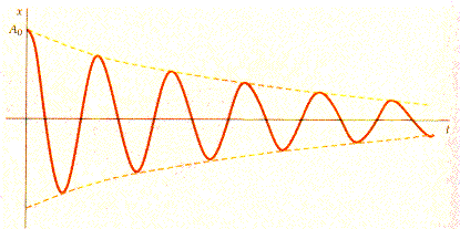
(2.3) x = Aexp(-bt)sin(at + f)
where
(2.4) b = c/2m
(2.5) a2 = w02 - b2
(2.6) w02 = k/rn
(2.7) k = k1+k2
This (2.3) is a sine wave in an exponential envelope. While the second term oscillates, it is multiplied by the first term which becomes smaller with time. The constant b is called the decay constant.
Experiment 2A. Measure the displacement vs time of the oscillation with the ultrasonic motion sensors. Verify that the amplitude of oscillation of the damped harmonic oscillator decays exponentially and determine the damping constant b for both cases of 1 and 2 magnets providing the damping. Fit the entire data set (a non-linear, least-squares fit) to Equation 2.3 (plus a constant since equilibrium is not zero in your data) using Excel, MathCad, Axum, Origin, or some other program of your choice. In Excel you would use the Solver. See the link at the top on how to use Solver to curve fit. A sample data set is included so that you can work on this part before you actually take data. The sample data set is in Excel format: right-click on this link and "save target as" so that you may download to your local computer and work on it.
Experiment 2B. Test whether the period of the oscillations is given by a (Equation 2.5), rather than by w0. You can obtain the period from the same graphs used to read off the amplitude of the oscillations during damping. The value of w0 was obtained in Experiment 1. If for Experiment 2A you do a fit to the entire data set, you will obtain the period automatically.
Part 3. Driven (forced) harmonic oscillator.
The system is driven if energy is imparted to the harmonic oscillator continuously by an external force. If you drive the oscillator sinusoidally, Dsin(wt), the system will show resonance when the frequency of the driving force is close to the natural frequency w0 of the unforced oscillator. Set up the harmonic oscillator as shown in the diagram below, with the Daedalon Precision Sine Drive anchoring one of the springs.

The net force on m is then given by
(3.1) F = - kx - cv + Dsin(wt)
The differential equation is thus
(3.2) mx'' + cx' + kx - Dsin(wt) = 0
The solutions are of the form
(3.3) x = Aexp(-bt)sin(at + f) + Bsin(wt - q)
provided the damping coefficient c is small. The first term is a transient term whose constants have been defined in Section 2. Notice that this term only lasts a certain amount of time, after a long enough time, t, the first term goes to zero and the system finds its steady-state. This makes sense: as you start to shake the system, it responds immediately, but takes a while to respond consistently to your shaking. The second term is the steady-state response, and describes the motion of the system after it settles down. In order to satisfy the differential equation (3.2), you can find B:
(3.4) B = D/{m[((w2 – w02)2 + 4b2w2)1/2]}
B is the amplitude of the steady-state motion. Note that B varies with the driving frequency.
Note that equation 3.4 simplifies to our other results, 2.3 and 1.5, if the constants are chosen appropriately.
Exercise 3.1: Using Equation 3.4, determine theoretically the value of driving frequency for which B a maximum. What is the amplitude of the motion at this frequency? When your driving frequency is at this frequency, it is called resonance, and the frequency is the resonant frequency. Resonance is an extremely important concept in many fields of science.
The diagram below shows a plot of amplitude vs. frequency for a forced harmonic oscillator. Low damping gives a sharper peak (the resonance peak is said to have a high Q), while more damping gives a wide peak (low Q).
Experiment 3A. Measure the amplitude of the oscillation (simply with the measurements given on the track) of the glider in the absence of magnetic damping, for frequencies w from 0.5w0 to 1.5w0. Although you can take data every 0.1 Hz far from resonance, it is advised that you obtain points at closer intervals near the resonance so that you do not miss the peak! Make note of the phase of x relative to the phase of the driving force when w<w0 and when w> w0.
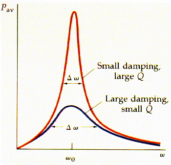
The left axis is the amplitude of the motion.
Experiment 3B. Repeat 3A but with a single magnet providing damping. (The damping is too great with 2 magnets. Remember you should always be leaving both magnets on the cart to keep the mass the same throughout the trials).
In your writeup of part 3, try to relate the shape of the resonance curves to Equation 3.4 - make sure it looks like expected - using the values of the constants w0 and b previously obtained in Experiments 1 and 2. One way to do this is to use the computer to plot Equation 3.4, using experimental values of the constants, on the same graph as the resonance curve data observed in 3a and 3b.
SKIP TO PART 5 (OR 4 IS OPTIONAL)
Part 4. Transient behavior at resonance.
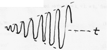
In the limit of undamped harmonic motion driven at the resonance frequency, the amplitude of the oscillations increases linearly with t without limit as more and more energy is transferred from the driver to the oscillator. This is why some seemingly very sturdy structures have been known to fall down.
Experiment 4. Using the ultrasonic measurement system, obtain a plot of glider position vs t at resonance, starting up from a stationary glider at the equilibrium position. Test whether the amplitude increases linearly, at least initially. Question 1: What is the rate of energy transfer to the glider? Is it a constant? If not, why not? Recall that the energy of a harmonic oscillator is proportional to the square of the amplitude of oscillation. Question 2: Why does the amplitude not increase without limit?
Driven oscillator with 2 masses.In many problems of interest to physics and engineering, one has not a single m but a collection of several m’s connected to one another by elastic forces. Example are vibrations of the nuclei in molecules or in crystals, or in spans which are parts of bridges. Classically, such systems have normal modes which are resonances of the combined system. There may be more than one normal mode resonance, and sometimes they are hard to find. For a one-dimensional system, there are as many normal modes as there are masses. We will measure the resonance curve for two masses connected by three springs, as shown below. The individual masses and springs will be identical to those used in the previous experiments. Assume for simplicity that k1 = k2 = k3 = k0.

The two-mass harmonic oscillator has two normal modes, called the symmetric and antisymmetric modes. In the symmetric mode, both masses move away from the center of mass; the center of mass does not move. In the antisymmetric mode, the two masses move to the left or right together, so that the center of mass oscillates about its equilibrium position. If driven by an external sinusoidal driver, the system will show resonances at the frequencies of these normal modes.
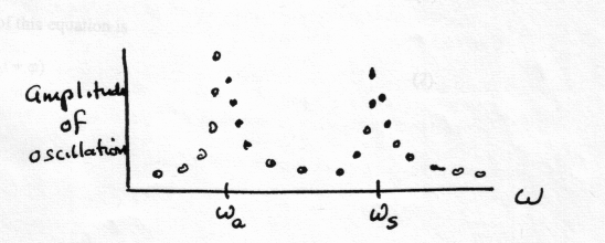
If the springs in the system are matched, so that k1 = k2 = k3 = k0, the frequency of the symmetric mode is
(5.1) ws = (3k0/m)1/2
while that of the antisymmetric mode is
(5.2) wa = (k0/m)1/2
For comparison, the frequency of the single glider is
(5.3) w = (2k0/m)1/2
Experiment 5a. Measure the amplitude of the resonance curve (like hand-drawn plot, above - vary driving frequency through the resonances and take amplitude data every so often) for two gliders and three springs separated by about 65 cm total from the left end of the left-hand spring to the right end of the right-hand spring. You will need to use a little skill in finding the resonance frequencies. When you find each, note the difference in the relative motion of the two masses at the two resonances. Check that the resonance frequencies agree with expectations (Equations 5.1 and 5.2).
The End