Diffraction Patterns

Equipment 

• Light meter on traveling stage:

  • Vernier 3-Level Light Meter

  • PASCO Rotational Motion Sensor

  • Linear Translation Stage

  • Aperture Bracket

• HeNe Laser

• Single slit, double slit, multiple slit brackets 

• CD-ROM

Theory

Recall that if two waves meet at a point they will interfere. The interference pattern will have a time averaged intensity (a photodetector or your eye averages the incident intensity over time) which is dependent on the relative distance from each source:

(1)   

where j is the phase difference between the two beams with wavelength l, ,

and the pathlength difference of the two beams is .

Where 's' is the distance between the two sources initially (the slit separation for a laser going through a double-slit.)

Exercise:  You should derive Equation 1.  If you look back to your first year text, you will see that it is pretty straight forward, and requires about 3 steps.

A double-slit pattern acts as two sources of light which spread out and interfere at multiple positions along a screen.  If the two sources had constant intensity vs. position, the intensity of each spot of constructive interference would be the same.  To the contrary, the light coming from a single slit with width 'a' has an intensity that varies with position with following result from single slit diffraction: 

(2)   

so the double slit diffraction pattern will have spots which vary with intensity as you move along the screen.  You need not derive Equation 2.

Procedure

Setup for Diffraction of light by N-slits.  

We are going to shine a laser through some slits, and project the resulting diffraction pattern some distance away.  We want to use a light meter (photometer) to measure the intensity of the light at various positions so that we can reproduce the light pattern as a plot of intensity vs. position.  We do this by allowing the light to fall on a small aperture (that only lets the light through at a particular position), and then we move the aperture to measure the light at other positions.  We have the aperture attached to a linear stage, which is moved using the Rotational Motion Sensor, so that it can be moved carefully and smoothly, and so the position can be recorded by the computer.

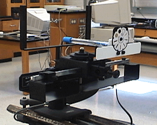
This is the linear stage with all the components.  Hover with your mouse to see what is what.

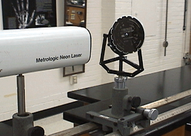
This is the laser and Slit Bracket.

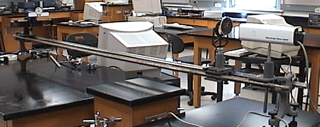
This is the whole setup, with the translation stage a bit difficult to see at the far end.

If the light meter on the traveling stage is not already setup for you, then you need to do the following (refer to the diagrams):

1. Insert the toothed bar of the Linear Stage through the appropriate hole in the Rotational Motion Sensor (RMS).  

2. Attach the Aperture Bracket to the rotational motion sensor, so that when you rotate the wheel on the RMS, the Aperture Bracket sweeps linearly, perpendicular to the direction of light entering the aperture.

3. Affix the Linear stage in place, perhaps on an optics rail.

4. Affix the Light Sensor to the back of the Aperture Bracket, so that light entering the aperture goes straight into the light sensor.  This is not trivial, as the two pieces of equipment were not made for each other.  It seems to be easiest to just do it with tape.  You may want to try adjusting the position of the light sensor between tries of taking data so that you can see if there is an optimal position.

5. At some distance away (at least 1-2 meters) from the Aperture Bracket, set the laser in place (on the optics rail) so that you can sweep the aperture past the laser beam.

6. Between the laser and aperture, affix the multiple slit bracket so that the diffraction pattern is over the aperture.

7. Now you can sweep the aperture across the diffraction pattern.  As you sweep, the light sensor records intensity and the rotational motion sensor records position, so you can reproduce the diffraction pattern as a plot of intensity vs. position.

Aperture Bracket and Slit Brackets

• You will want to experiment with the size of the aperture that allows you to take the best looking data.

• You will be asked to try various different numbers of slits, but to take data for comparison to theory, you should choose any double slit pattern.  Be sure to record the slit width 'a' and the slit separation 's' (sometimes the slit separation is also called 'd').

Computer Setup

Attach the Light Sensor and Rotational Motion Sensor to the Vernier ULI (old interface, need to attach it to the computer) as follows:

1. The Light Sensor should be set on its most sensitive scale, and plugs into the DIN1 input.

2. The Rotational Motion Sensor should plug into the PORT2 input.

3. Be sure that the ULI is on and start up LoggerPro data acquisition program.

4. In LoggerPro, make sure (Setup-Interface) that it is reading the ULI interface plugged into whatever port you plugged it into in the back of the PC.

5. We will setup the program to record data from the sensors first by setting the Sensor Properties under the Setup menu.

6. Click on the DIN1 port and choose the Light Sensor-600 (make sure the light sensor is set on 600) as the Sensor.
   

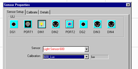
7. Click on the PORT2 input and choose the Rotary Motion (Pasco) sensor.  In addition, you want to choose the appropriate calibration file for this experiment.  Since we are using the RMS (rotary motion sensor0 to measure linear distances, you must choose the position (PRMPosX4) calibration rather than one for angle.

8. Go to the Details tab to make sure it is setup correctly; in particular, be sure to change the Diameter of the RMS to be 30.  Check that all the other parameters match up as below.
   

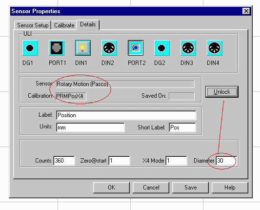
9. When you are finished setting up the sensors, you can tell the computer how fast to take data.  Go back to Setup - Data Collection.  There are 3 parameters you will want to adjust to try to find the optimal way to take data.  The first is just experiment length.  This is unimportant just so long as it is long enough for you to be able to sweep across the whole diffraction pattern.  If you set it as a long time, then you will only need to hit the Stop button when you are done taking data.  The two meaningful parameters are how fast you take data (sampling speed) and how many data points you average for one displayed data point.  Initially you can leave these as you found them, but you may want to go back later and adjust these to see if you can take a better set of data.
   

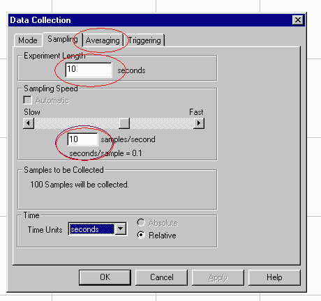
10. You are now ready to setup the display of the data.  You want to plot intensity vs. position.  An empty graph should be displayed on the screen.  Click on the y-axis label, and a box should pop up giving you a choice of what to display.  Choose the appropriate variable, and then do the same for the x-axis label.

11. You are finally ready to take data.  At any time you can hit the Collect button to start taking data.  When you are finished you can click the Stop button.  

Taking Data

• Sweep the aperture across the diffraction pattern and the computer will record intensity and position.  The sweep will be done by hand, by carefully rotating the wheel on the RMS.  You might try to sweep across a large portion of the pattern, but the edges might be too dim to warrant much effort.  Be sure to at least get a good sweep of the central bright part of the pattern.

• If the data does not show up on the graph, yet you see numbers in the spreadsheet, it is simply a problem of scale.  To rescale, you click on either axis and choose Autoscale.  

• If you don't get any readings different from zero, make sure everything is on and that the Light Sensor and Aperture Bracket are appropriately positioned. 

• In order to get the best looking data you can, remember to adjust aperture size, sensor position, rate of sweep, smoothness of sweep, sampling speed and averaging.

Experiment:

Preliminary measurement.  Project the laser through the slits and observe the pattern.  Experiment with the pattern by changing from 1 to 2 to n slits. Describe what you see.

Detailed scan.  Make a detailed scan of a double-slit pattern, plotting the intensity vs. position.  Using this plot, make estimates of the slit width 'a' and separation 's', with errors.  (Hints: you can find 's' by using Equation 1, and determining the distance between adjacent constructive interference spots; you can find 'a' by using Equation 2 and finding the distance between two places where I_q = 0, that is where there are no interference spots because there was no intensity; you can relate your position variable to q only if you know the distance from the slits to the detector.) 

Computer analysis.  Combine Equations 1 and 2 to create an equation which should describe your double-slit data.  You do this by realizing that I₀ in Equation 1 is actually not a constant intensity, but varies with position, as given by Equation 2.  So you can plug in I_q from Equation 2 as I₀ in Equation 1.  I₀ in Equation 2 represents the actual incident intensity.  You can do a least squares fit in your favorite piece of software (perhaps Excel's Solver), allowing the parameters 'a', 's', and 'I₀' to vary.

Laser Lab Home    Speed of Light    Diffraction    CD-Diffraction